Some notes about Discrete-time systems
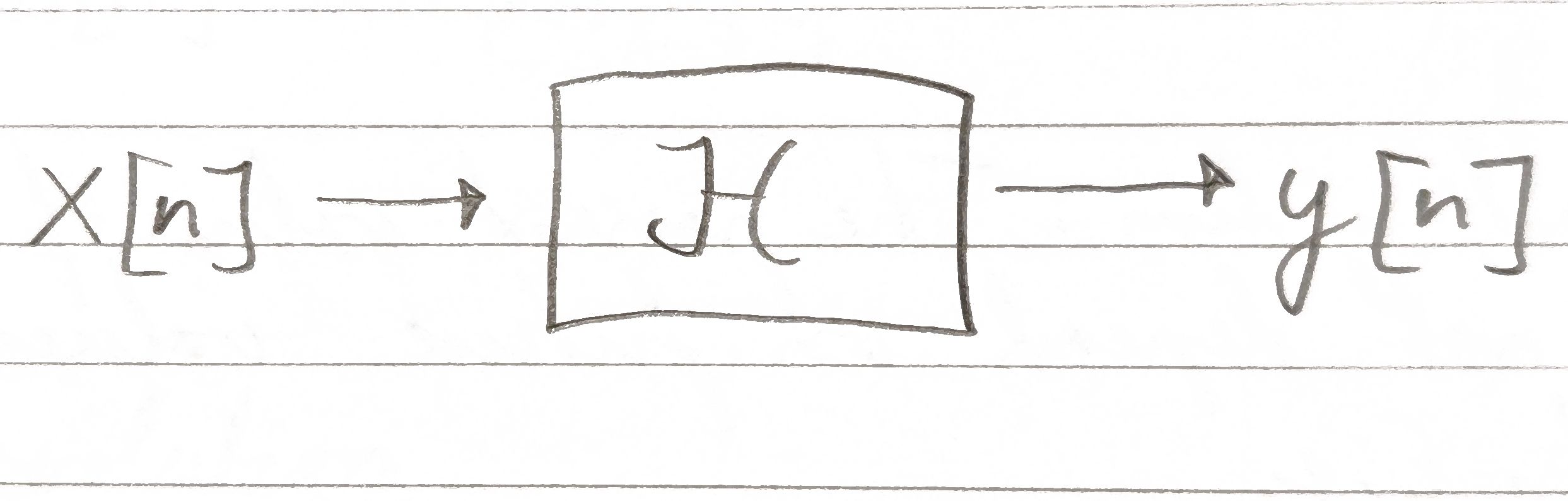
In the field of Digital Signal Processsing a discrete-time system is a computational process that takes any signal $x[n]$ and produce a signal $y[n]$, here $y[n]$ is called the output signal. We typically denote this process as $H$, and we say that $x[n]$ maps to $y[n]$ by operator $H$. This is all very fancy language, and basically all we are saying is that we have some algorithm, that we can assert on our signal $x[n]$ which will produce $y[n]$. This is illustrated by our picture below.
This is a very general definition, basically it is almost all mathematical operations. To be able to create general rules which apply for all discrete-time systems is hard, and hence the usefullness of discrete-time system is limited. In Digital Signal Processing we therefore typically focus on a sub-class of these systems that satisfy some or all of the following properties. If they satisify these conditions, as we will see, we can analyse these systems in much more details. These properties are:
Causality
If the present value at the output of $H$ does not depend on future values of $x[n]$, the system is said to be casual. This definition is so trivial that it can be confusing. To give a very simple example of a noncasual system: $$y[n] = x[n+2]$$ Think about how you could construct this if you did not have the complete signal $x[n]$? That is, you see one input coming at a time. You get the input sample $x[n]$, you then somehow need to set $y[n]$ equal to the sample $x[n+2]$, a sample you have not recieved yet! It should be noted that this is not a problem for a signal where all samples are stored in memory.
Mathematically we can write it as: $$x[n] = 0 \ \text{for}\ n \leq n_0 => y[n] = 0 \ \text{for} \ n \leq n_0$$ If $x[n]$ is zero for all $n \leq n_0$, then $y[n]$ must also be zero for the same $n$. This would not be the case for a noncasual system.
Stability
Stability is just saying that for any $x[n]$ we do not want the output $y[n]$ to go to infinity. This is an obvoius condition if we are suppose to analyse the signal on a computer.
Linearity and time invariance
While stability and causality are nice to have properties to be able to create a discrite-time system, the linearity and time invariance property is required to be able to mathematically analyze it. A system is said to be linear if and only if the following holds: $$H ( ax_1[n]+bx_2[n] ) = H( ax_1[n])+H(bx_2[n])$$
It is usually quite straight forward to prove/dis-prove if a system is linear or not. You can plug in $x_1[n] + x_2[n]$ into $H$ and see if you get the same as if you plugged them in seperatly. However, sometimes it is not so easy, at least I think so. Take for instance the following difference equation: $$y[n] = x[n]+2*y[n-1]$$
Lets say you set $x[n] = x_1[n] + x_2[n]$, this gives:
$$y[n] = (x_1[n]+x_2[n])+2*y[n-1]$$
But what should you put in for $y[n-1]$? We have not really proven that the difference equation is linear yet, so putting in $y_1[n]+y_2[n]$ would not be logically sound. It would be cheating in my opinione. Let’s do it the other way around, we have the following two equations:
$$y_1[n] = x_1[n]+2*y_2[n-1]$$
$$y_2[n] = x_2[n]+2*y_2[n-1]$$
Then lets ask ourselfs what input we have for $y_1[n]+y_2[n]$. This gives:
$$y_1[n]+y_2[n] = x_1[n]+2y_1[n-1] + x_2[n]+2y_2[n-1]$$
$$= (x_1[n]+x_2[n])+2*(y_1[n-1]+y_2[n-1])$$
Yey. We have proved that the difference equation is linear.
Time invariance is just saying that the characteristics of a system does not change with time, or sample index. This is also quite trivial. But inportant. Not all system have this property.