DFT and Autocorrelation
DFT - Descrete Fourier transform
Here is the definition of the DFT (exactly as the python library Numpy defines it):
$$X[k] = \mathcal{F}(x[n]) = \sum_{n=0}^{N-1} x[n]e^{-j2\pi nk/N} $$
As you see here, I’m using capital letters to illustrate the DFT of some sequence. That is $Y[k] = \mathcal{F}(y[n])$. I will use this throughout the text. If you want to read more about the DFT, check out mye page here (link).
Autocorrelation
Autocorrelation of some sequence $x[m]$, with length $N$, is defined as the sequence:
$$r[m] = \sum_{n=0}^{N-1} x^*[n]x[n+m]$$
here $x^* [n]$ is the complex-conjugate, and $m$ is in the range $0$ to $N-1$. One more thing we should specify here is what happens with the last part $x[n+m]$ when $n+m>N$. How do we define $x[n]$ out of its bound? It is common to assume that $x[n]$ is periodic with period $N$. That is $x[n+N] = x[n]$. As we will see, we will need this later on.
Wiener-Khinchin Theorem
This theorem states that the DFT of the autocorrelation sequence $r[m]$ is equal to the power spectrum of $x[n]$. Written out this becomes:
$$ R[k] = \mathcal{F}(r[m]) = |X[k]|^2.$$ To me at least this is not a trivial result. So lets prove it.
Wiener-Khinchin Proof:
We start by taking the DFT of the covariance function $r[m]$.
$$ R[k] = \mathcal{F}(r[m]) = \sum_{m=0}^{N-1} r[m] e^{- j 2 \pi m k/N} = \sum_{m=0}^{N-1} \left(\sum_{n=0}^{N-1}x^*[n]x[n+m]\right) e^{- j 2 \pi m k/N} $$
All we have done above is using the definitions for the DFT and $r[m]$. Now in the last summation, since $x^*[n]$ is independent of the index $m$ we can write the last summation as:
$$ \sum_{m=0}^{N-1} \left(\sum_{n=0}^{N-1}x^*[n]x[n+m]\right) e^{- j 2 \pi m k/N} $$
$$ = \sum_{n=0}^{N-1} x^*[n] \left( \sum_{m=0}^{N-1}x[n+m] e^{- j 2 \pi m k/N}\right) $$
This trick is not so easy to see by just looking at the equation. But if you try to write out the sum you can more easily see it.
Now since the inner term $x[n+m]$ always starts iterating at index $n$, which is fixed for the whole inner summation, we can write the inner sum like this: $$ = \sum_{n=0}^{N-1} x^*[n] \left( \sum_{m=n}^{N-1+n}x[m] e^{- j 2 \pi (m-n) k/N}\right) $$
$$ = \sum_{n=0}^{N-1} x^*[n] \left( \sum_{m=n}^{N-1+n}x[m] e^{- j 2 \pi m k/N}e^{ j 2 \pi n k/N}\right) $$
$$= \sum_{n=0}^{N-1} x^*[n]e^{ j 2 \pi n k/N} \left( \sum_{m=n}^{N-1+n}x[m] e^{ -j 2 \pi m k/N}\right) $$
Now for the trick we promised to use (see Autocorrelation)! Since we assumed $x[n+N] = x[n]$ we can write the inner sum as:
$$ = \sum_{n=0}^{N-1} x^*[n]e^{ j 2 \pi n k/N} \left( \sum_{m=0}^{N-1}x[m] e^{ -j 2 \pi m k/N}\right) $$
The inner sum is now independent of the outer summation and can be “pulled out”, leaving us with:
$$ = \left( \sum_{n=0}^{N-1} x^*[n]e^{ j 2 \pi n k/N} \right)\left( \sum_{m=0}^{N-1}x[m] e^{ -j 2 \pi m k/N}\right)$$
$$ = \left( \sum_{n=0}^{N-1} x[n]e^{ -j 2 \pi n k/N} \right)^*\left( \sum_{m=0}^{N-1}x[m] e^{ -j 2 \pi m k/N}\right) $$
$$ = X^*[k]X[k] = |X[k]|^2 $$
QED.
Now if you found the math above a bit cumbersome, here is some Python code proving that they are equal for some arbitrary signal:
def autocorrelation(x, mode="periodic"):
""" Does the auto correlation of a signal X with no scaling
mode -- If 'periodic' x is assumed to repeat every N = length(x)
If 'zero' x is assumed zero out of its bound
"""
N = len(x)
# Check if complex or not
if np.iscomplexobj(x):
comp = True
acorr = np.zeros(N)+1j*np.zeros(N)
else:
comp = False
acorr = np.zeros(N)
# Check mode
if (mode=="periodic"):
x_per = np.concatenate([x,x])
else:
x_per = np.concatenate([x,np.zeros(N)])
# Do autocorrelation
for k in range(N):
for n in range(N):
if comp:
acorr[k] = np.conjugate(x[n])*x_per[n+k] + acorr[k]
else:
acorr[k] = x[n]*x_per[n+k] + acorr[k]
return acorr
# Create an arbitrary signal
start = 0
step = 0.001
Freq = 14
Freq2 = 50
N = 1000
t = np.arange(0,N)*step+start
# Create a complex signal
x = 20*np.exp(1j*2*np.pi*Freq*t) + 10*np.exp(1j*2*np.pi*Freq2*t)
## Proof
# Calculate DFT of autocorrelation
r = autocorrelation(x)
r_fft = np.fft.fft(r)
# Calculate Power of the DFT
x_fft = np.fft.fft(x);
x_psd = np.abs(x_fft)**2
# Plot
plt.figure(1)
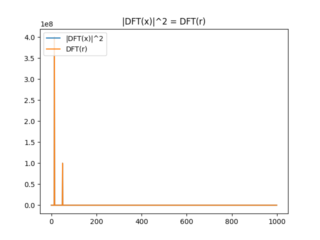
plt.title("|DFT(x)|^2 = DFT(r)")
plt.plot(x_psd, label='|DFT(x)|^2')
plt.plot(r_fft, label='DFT(r)')
plt.legend(loc="upper left")
plt.show()
Running this code gives you the following plot:
Summary
This section can be summed up with the following diagram. The point I want to make is this: the power spectrum of some sequence $x[n]$ is exactly the same as the DFT of the autocorrelation function.
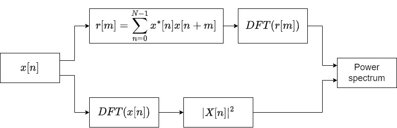
Now you may ask, “Why do we want to do it one way or the other?”, “How does this relate to the MUSIC algorithm?”. I will try to answer these question in the following sections. For now, just remember this property.